
GET TO KNOW THE STEPS OF MAPBIOMAS METHODOLOGY
Here we detail the Mapbiomas methodology step by step. For each class and theme treated in the map there are specific perculiarties and characteristics that can be checked in detail in the ATBD in its appendices.
DOWNLOAD THE COMPLETE METHODOLOGY - ATBD
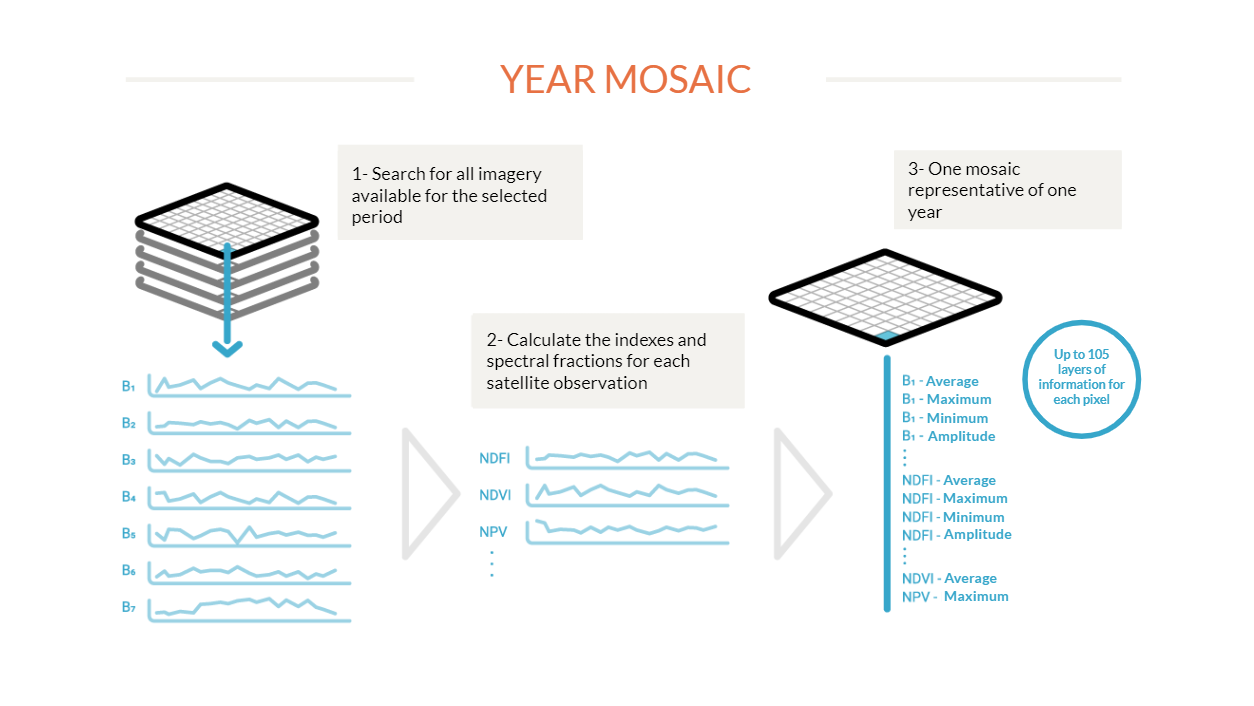
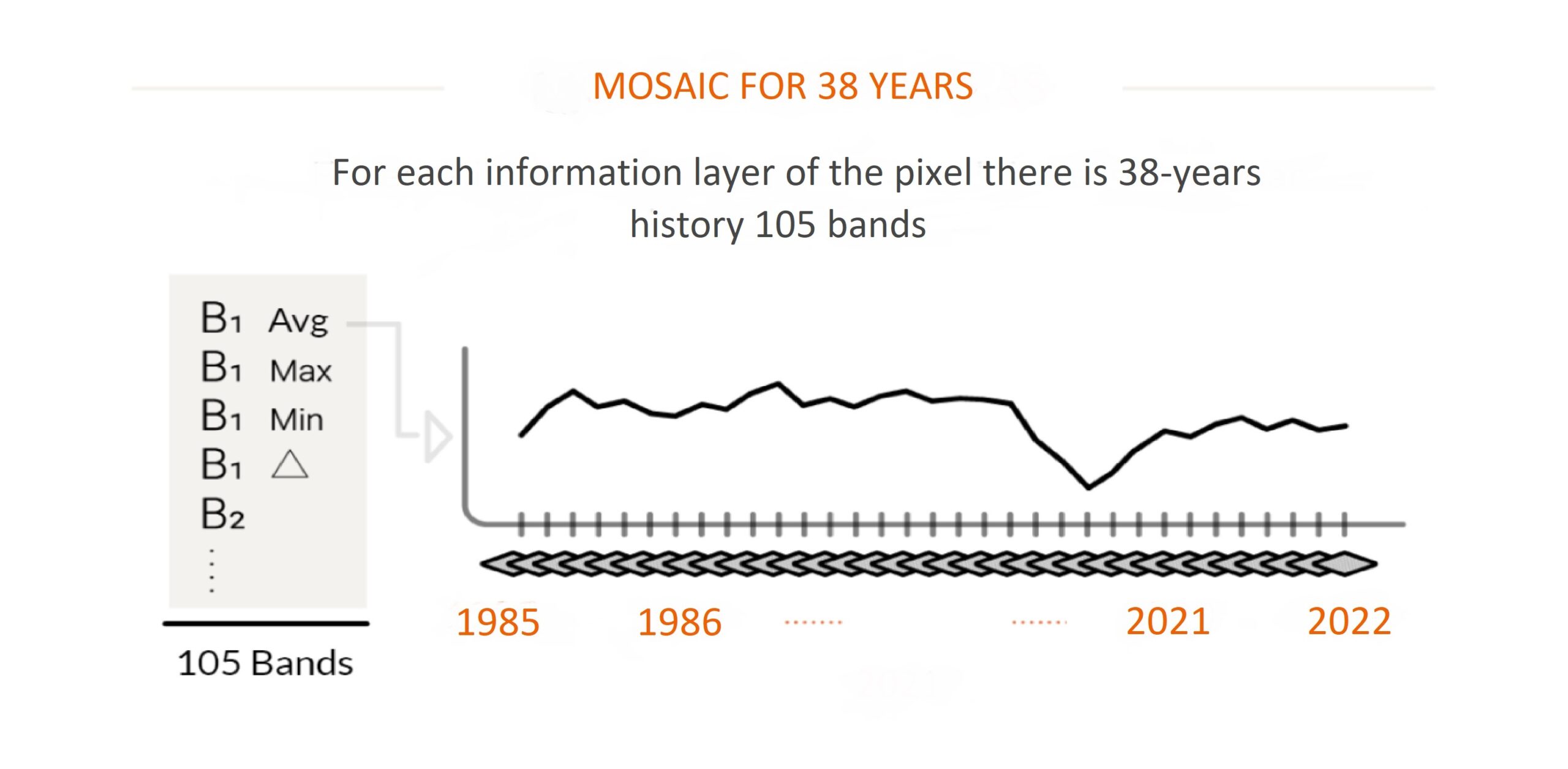
It all starts with Landsat satellite imagery, with 30-meter resolution, available for free on the Google Earth Engine platform and with a time series of more than 30 years. It takes 380 Landsat images to cover Brazil, each with tens of millions of pixels: in total, there are more than 9 billion pixels of 30 x 30 meters to make up the entire country. These pixels are the MapBiomas working units. Images can contain clouds, smoke, and other artifacts that can "dirty" them. To produce a clean image, the cloudless pixels are selected from the available images for the selected period. For each of these pixels are extracted metrics that explain the behavior of the pixel in that year. This is done with each of the 7 satellite spectral bands as well as for the calculated spectral fractions and indexes. For example, for Band 1 the median of band values in the period, the maximum value, the minimum value in the year and the amplitude of variation is collected. At the end each pixel for one year carries up to 105 layers of information.
For each year a mosaic covering Brazil is set up representing the behavior of each pixel through 105 metrics or layers of information. This mosaic set is saved as a collection of data (Asset) within the Google Earth Engine platform. These mosaics will be used in two main ways. First as source parameters for the algorithm to produce classification (see next step). It is also from this mosaic that RGB composition is derived allowing to visualization of the background image in the platform MapBiomas. This composition is also used for the collection of training samples and samples for assessment of accuracy by visual interpretation.
From the image mosaics, the teams of each biome and each cross-sectional theme produce a map of each land cover class (forest, field, agriculture, pasture, urban area, water, etc). To do so, MapBiomas analysts use an automatic classifier called "random forest", which runs on Google Earth Engine. This system is based on machine learning: for each topic to be classified, the machines are "trained" with samples of the targets to be classified. These samples are obtained by means of reference maps, generation of maps of stable classes of the previous series of MapBiomas and by direct collection by visual interpretation of the Landsat images. The classification is made for each of the years of the series and can be saved as a single map per class where each pixel has the number of layers corresponding to the number of years of the analyzed historical series.
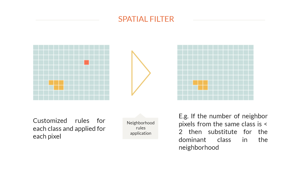
The spatial filter aims to increase the spatial consistency of the data by eliminating isolated or border pixels. Neighborhood rules are defined that can lead to a change in pixel classification. For example, a pixel that has less than two out of the nine neighboring pixels in the same class will be reclassified to the predominant class in the neighborhood. Each pixel in each year and for each class of use is subjected to spatial filtering.
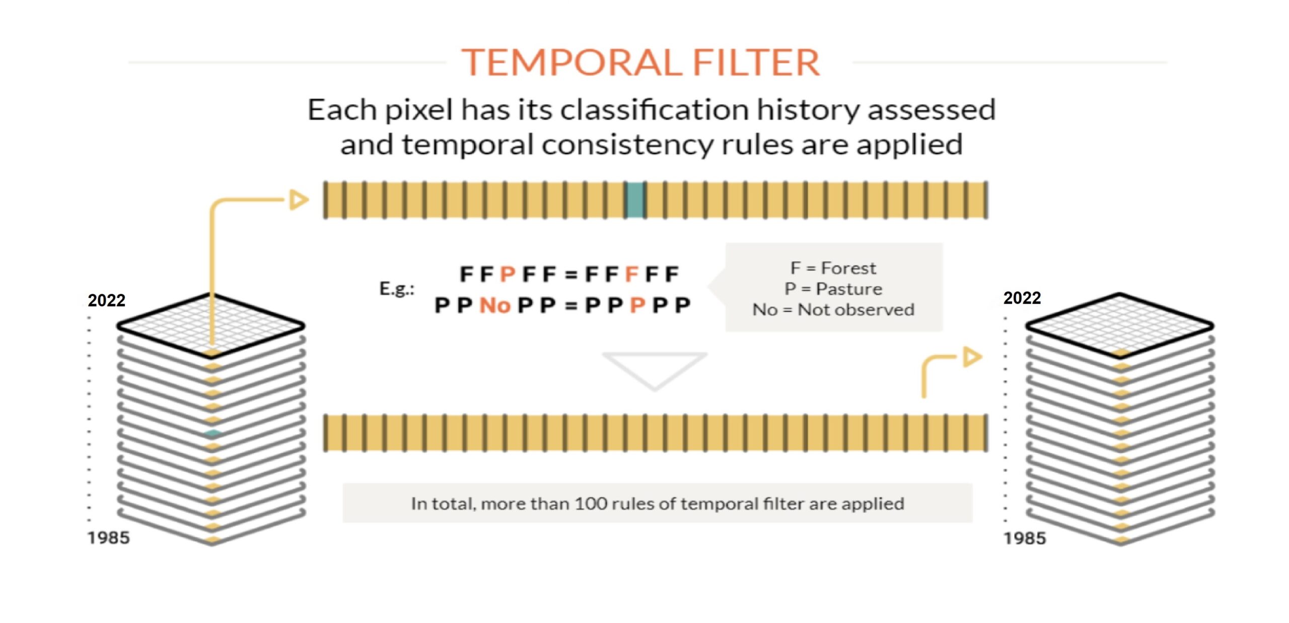
In order to reduce temporal inconsistencies, in particular changes in coverage and use that are impossible or not permitted (eg Natural Forest > Non-Forest > Natural Forest) and to correct failures due to cloud overflow or lack of data, a temporal filter is applied. Each biome, theme or region may have specific temporal filter rules. In total in Collection 3 more than a hundred rules have been applied. The temporal filter is applied to each pixel analyzing all the years of the Collection (eg Collection 8 were 38 years).
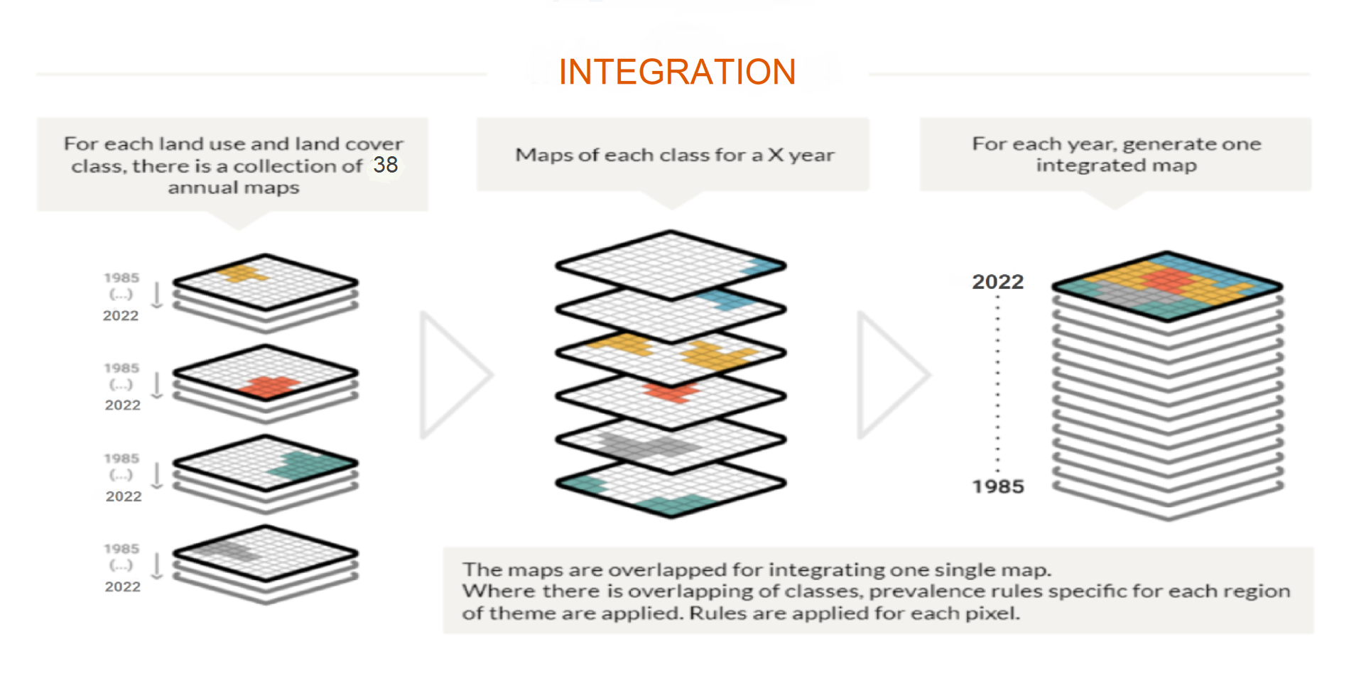
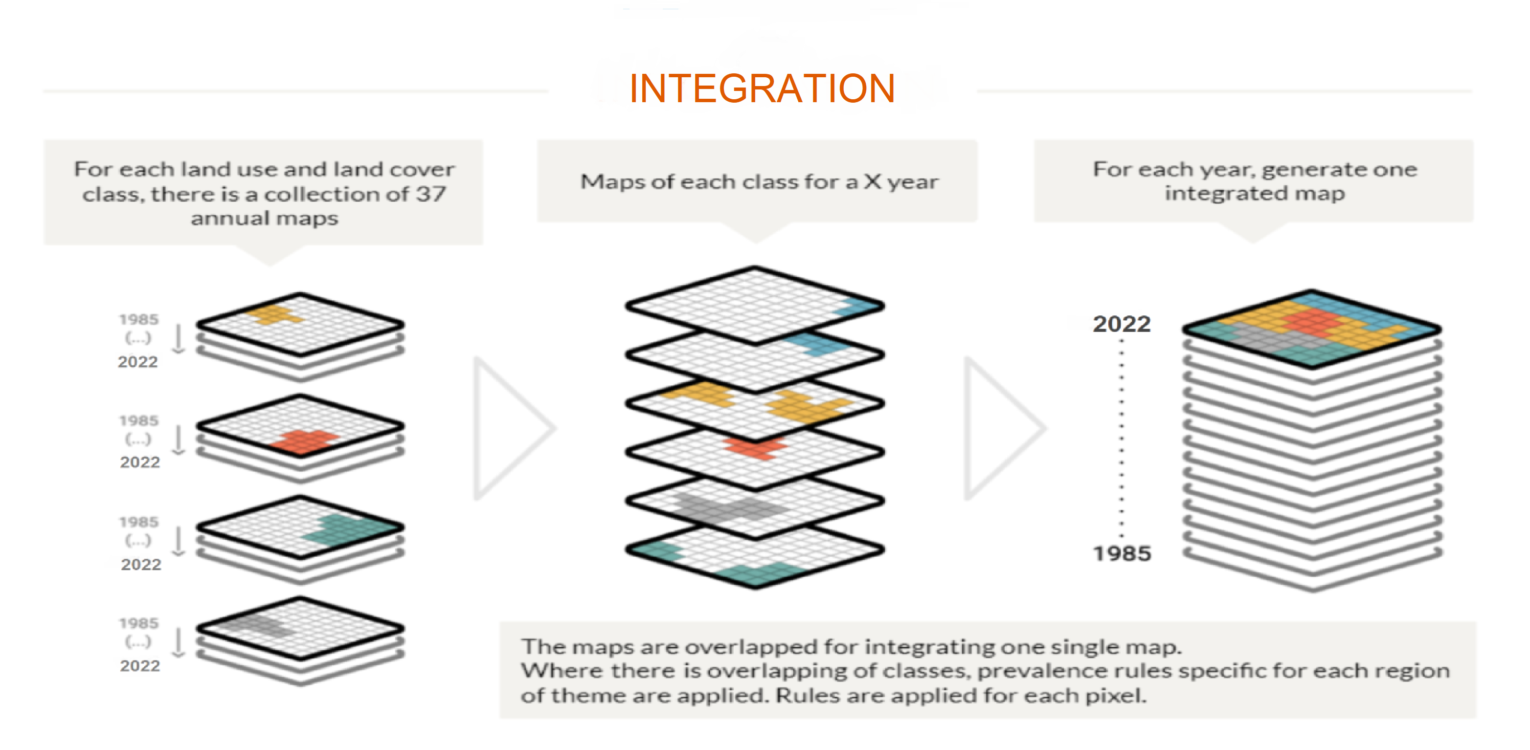
In this step, the maps of each class are integrated into a single map, which represents the coverage and land use of each territory for each year. Prevalence rules are applied: Thus, if the same pixel is classified into two distinct class maps, it is possible to define which one belongs to the final map. The prevalence rules may vary according to the peculiarities of the biomes, themes or regions. The integration is done for each year of the series and generates an integrated map for each year usually saved as a single ASSET with the number of annual layers of the period analyzed. The integrated map goes through a further step of spatial filtering to clean the edges and loose pixels as a consequence of the integration process.
In order to understand changes in land cover and land use, maps are produced with class transitions between different pairs of selected years. It is thus possible to visualize the dynamism of the territory, and answer questions such as how much of the forest has turned pasture from one year to another, for example, among other changes in the landscape. Transition maps are produced pixel by pixel and after finalized also pass through a spatial filter to eliminate isolated transition or border pixels. From these maps are constructed the transition matrices for each biome, state, municipality and other territorial courts available on the MapBiomas platform.